Signal Simulation Real R & Complex C – Telecommunications, Navigation & Electronics

Introduction

When I first started working with simulation software such as ScicosLab/Scicos fifteen years ago (Ref.1/2), I used Real signals. Later on when working with GNU Radio I discovered it was also possible to generate Complex signals. It is worth considering the differences between the two approaches.

Fourier Transform

Let’s do a quick review of the math involved in Real & Complex signals. Let s(t) be a telecommunications signal. The Fourier Transform and Inverse Fourier Transform are defined as:
F[s(t)] = S(f) = integral[s(t)*exp(-j*2*pi*f*t)*dt] -infinity,+infinity
s(t)= Finv[S(f)] = integral[S(f)*exp(j*2pi*f*t)*df] -infinity,+infinity
Now consider a signal s(t) = constant = A:
S(f) = A*delta(f), delta = Dirac Delta or Unit Impulse Function

A trigonometric function cos(wct) can be shown to be:
cos(wct)=0.5*[exp(jwct) + exp(-jwct)]
F[cos(wct)] = 0.5*[delta(f-fc) + delta(f+fc)]
Which represents two spectral lines one at f=fc and another at f=-fc.

Real Signals

Fig.2 GNURC Schematic Real Cosine Signal Freq=1KHz Amp=1 Spectral Line Level=-15dBr

Figure 2 shows a GNURC schematic generating a 1KHz Cosine wave with relative amplitude of 1. Since this is a real signal, we have two spectral lines one at -1KHz and the other at +1KHz at a relative level of approx -15dB. Adjusting the amplitude to 2, will increase the spectral line level by 20log10(2) = +6dB to -9dB.

Complex Signals

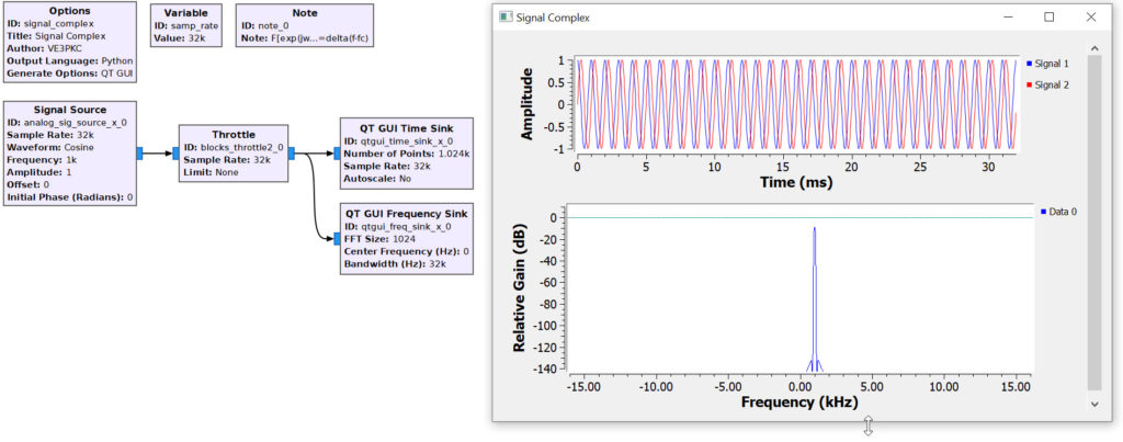
Fig.3 GNURC Schematic Complex Cosine Signal Freq=1KHz Amp=1 Spectral Line Level=-9dBr

Figure 3 shows a GNURC schematic generating a complex 1KHz Cosine wave [exp(jwct)] with relative amplitude of 1. Since this is a complex signal, we have only one spectral line at +1KHz at a relative level of approx -9dB. Adjusting the amplitude to 2, will increase the spectral line level by 20log10(2) = +6dB to -3dB. Note the scope blue signal is cos(wct) and the red signal is jsin(wct).

Mixing/Superheterodyne

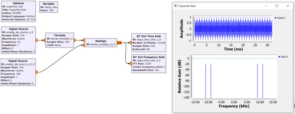
Fig.4 GNURC Schematic Showing Mixing Two Real Cosine Signals at 1KHz & 10KHz

Figure 4 shows a GNURC schematic showing the mixing of two real Cosine signals of 1KHz & 10KHz. The multiplication of two Cosine signals gives two components at the sum & difference frequencies of 9KHz and 11KHz as shown. Since they are Real signals they also have components at -9KHz & -11KHz.

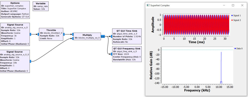
Fig.5 GNURC Schematic Showing Mixing Two Complex Cosine Signals at 1KHz & 10KHz

Figure 5 shows a GNURC schematic showing the mixing of two complex Cosine signals of 1KHz & 10KHz. The multiplication of two complex Cosine signals is equivalent to:
exp(jw1t)*exp(jw2t)=exp(j(w1+w2)t) or a single spectral line at 11KHz.

Gaussian Pulse In Limit

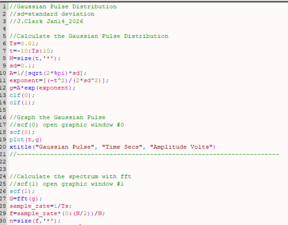
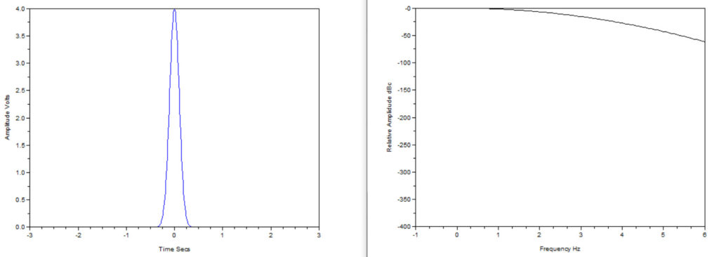
Fig.6 ScicosLab Script for Gaussian Distribution Pulse

Fig.8 Gaussian Pulse Time & Spectrum for SD=0.05

In Ref.3 I looked at how you can generate a Dirac Impulse by considering a rectangular pulse train in the limit. You can also do this by using a Gaussian pulse and varying the standard deviation. Figure 6 is a ScicosLab script to generate a Gaussian pulse. Figures 7/8 show how the pulse tends to a Dirac Pulse as the SD approaches zero.

gaussian_pulse.sce (zip file)