
Introduction
Costas & Squaring Loops are key components in reception of Telecommunication Signals. They are used to synchronize a local generated carrier with an incoming received carrier. We can simulate and study their operation using Scicos (Ref.1). First we generate a BPSK waveform at R=100bit/sec to use with our two Demodulators (Ref.2).
BPSK Waveform Generation
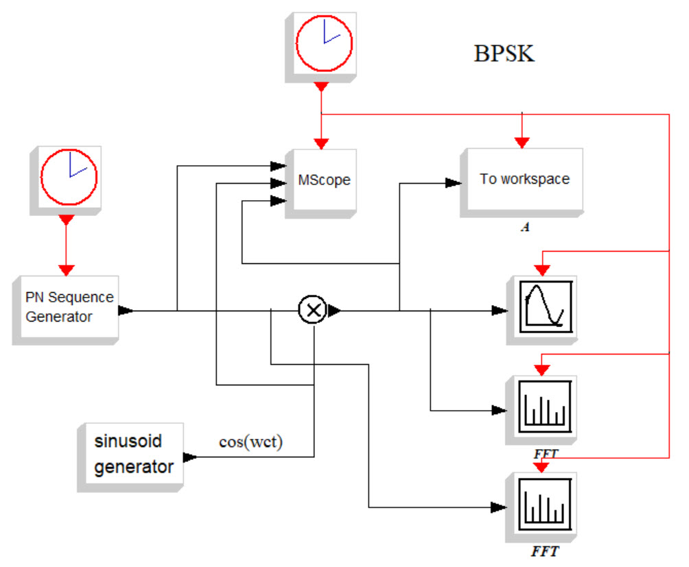
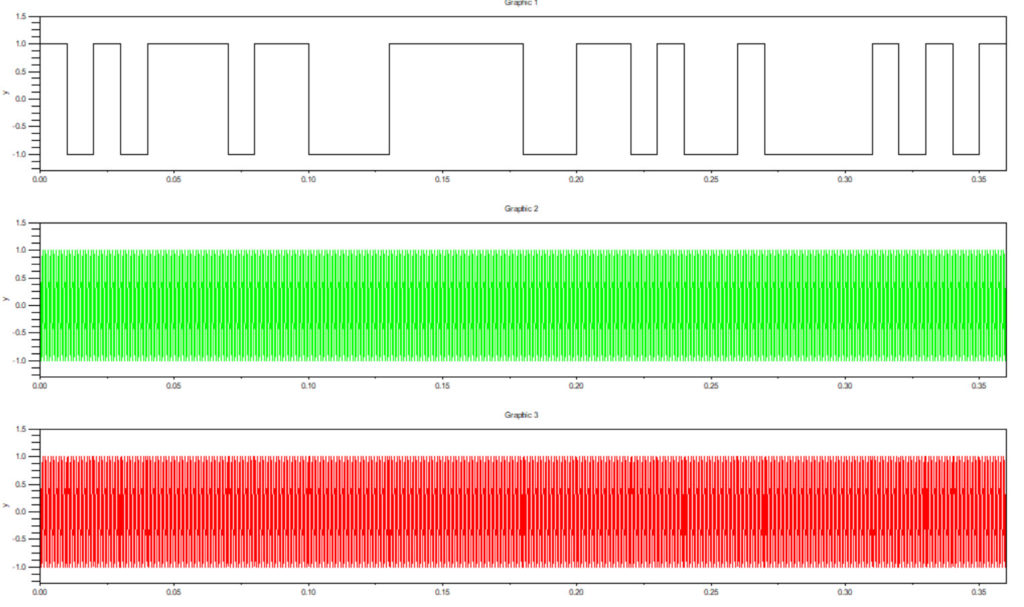
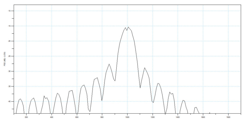
Figure 1 shows a Scicos Schematic that can be used to generate BPSK at R=100bit/sec with carrier Fc=1KHz. This is identical to the schematic used in Ref.2 for QPSK by just removing the Demux & Q branch. Figure 2 shows the PN data waveform repeating every 31bits=31*0.01sec=310msec. Figure 3 shows the output spectrum centered at Fc=1KHz +/-100Hz to first nulls. Notice the absence of a discrete line at Fc that a receiver could lock on!
Costas Loop Scicos Simulation
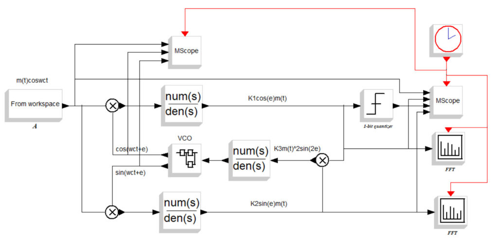
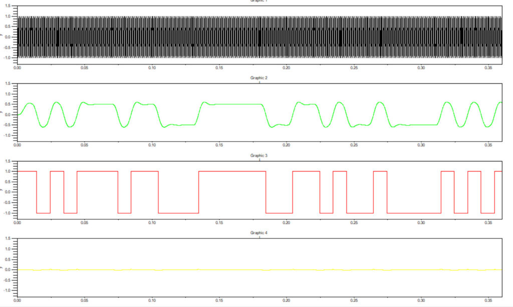
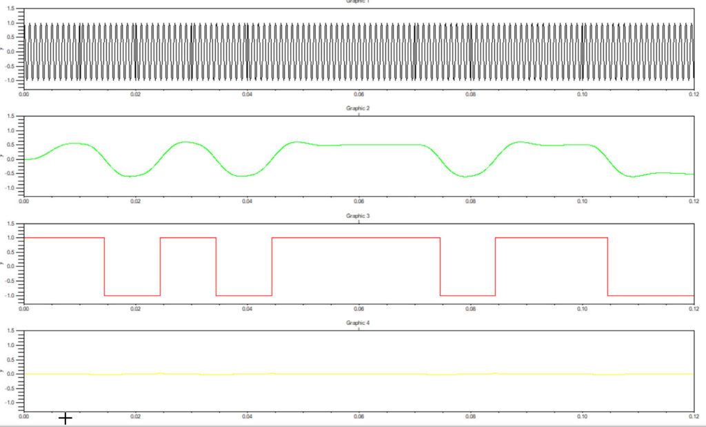
Figure 4 shows a Scicos Schematic for a Costas Loop BPSK demodulator. Following the derivation in Ref.3, assume that the VCO is almost locked to the incoming carrier with a small phase error of e. On the I branch:
m(t)cos(wct)*cos(wct+e)=0.5m(t)[cos(e)+cos(2wct+e)]
After the LPF (removes 2wct component):
m(t)cos(wct)*cos(wct+e)=0.5*m(t), (cos(e)=1 for small e)
On the Q branch:
m(t)cos(wct)*sin(wct)=0.5m(t)[sin(e)+sin(2wct+e)]
After the LPF (removes the 2wct component):
m(t)cos(wct)*sin(wct+e)=0.5m(t)sin(e)
On the VCO branch:
0.5m(t)cos(e)*0.5m(t)sin(e)=0.25(m(t)^2)sin(2e)
The VCO LPF picks out the DC component to drive the VCO.
Figures 5 & 6 show the demodulated BPSK data waveform identical to what was sent.
Squaring Loop Scicos Simulation
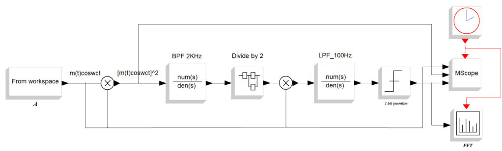
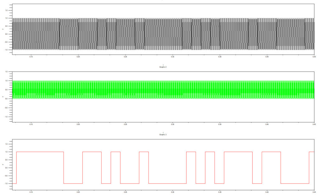
Figure 7 shows the Squaring Loop used for carrier recovery and data demodulation. The input signal is first squared:
[m(t)*coswct]^2=0.5*([m(t)]^2 + cos(2wct))
Thus this gives a low frequency component plus a perfect carrier at twice wc. This is then Band Pass Filtered to give just the carrier component at 2wc. Finally this is divided by 2 (not so easy!!!!) to yield a perfect version of the received carrier. Recall that the transmit spectrum had no discrete line at Fc! This recovered carrier now multiplies the input received signal and Low Pass Filtered to remove m(t)/2 as in the Costas Loop I Branch. Figure 8 shows the data recovery identical to what was transmitted.
Learn Telecommunications by Simulation
HF Radio Telecommunications Learn by Simulation
Please send your comments, questions and suggestions to:
contact:

References
#1. – “HF High Frequency Radio Telecommunications Learn by Simulation”
https://www.clarktelecommunications.com/simulation.htm
#2. – “Satellite QPSK/OQPSK Simulation “
https://jeremyclark.ca/wp/telecom/satellite-qpsk-oqpsk-simulation/
#3. – “Phase-Locked Loops Design & Applications”, 5th Edition, Roland E. Best
https://www.amazon.ca/dp/0071412018/